Adding Shapes: My Bachelor Thesis on Minkowski Sums

On 15 July 2019 I handed in my bachelor thesis, Berechnung der Minkowski-Summe für einfache Polygone (Calculating the Minkowski Sum of Simple Polygons). It is a fairly mathematical document, but the problem it solves has an appealingly physical interpretation: what shape do you get when you slide one shape over another and collect every position it can reach?

This post is the version I wish I had written alongside the thesis. It focuses on the central idea rather than reproducing all of the definitions, proofs, and implementation details.

The shape made by adding every point #

For two sets of points A and B in the plane, the Minkowski sum is

A ⊕ B = {a + b | a ∈ A, b ∈ B}

The addition is vector addition. Pick one point from each shape, add their coordinates, and the resulting point belongs to the sum. Repeating that for every pair fills the result.

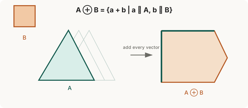
That definition is simple, but implementing it is not. There are infinitely many pairs of points, and even the finite set of polygon vertices does not tell us the whole answer by itself. The useful observation is that the boundary carries enough structure to construct the result.

This operation appears in places where geometry and algorithms meet:

• In motion planning, inflate obstacles by the robot’s shape. A point can then be planned around the inflated obstacles as if it were the robot.
• In CNC and 3D printing, combine the tool or nozzle shape with the object to obtain the path the tool must follow.
• In collision detection and image processing, use the same operation as a geometric form of dilation.

The easy case: convex polygons #

For two convex polygons, there are two natural algorithms.

The straightforward one forms every vertex sum vᵢ + wⱼ, then computes the convex hull. With n and m vertices, this creates n · m candidates before the hull algorithm removes the ones that cannot be on the boundary.

The better algorithm exploits the fact that the edges of a convex polygon are already ordered by direction. Start at the lexicographically smallest vertex of each polygon and walk around both boundaries. At every step, compare the direction of the next edge in each polygon and append the smaller direction to the result. If both directions agree, append their combined edge. Every input edge is consumed exactly once, so the running time is O(n + m).

This is a small but important algorithmic lesson: the geometry gives us an ordering for free. Once we use it, we no longer need to generate and sort all possible vertex pairs.

Why concave polygons change everything #

Concavity breaks that one-pass walk. The sum of two concave polygons may have indentations, several boundary components in intermediate constructions, and edges that overlap or intersect. A local choice of the next edge is no longer enough to tell us which parts will survive in the final boundary.

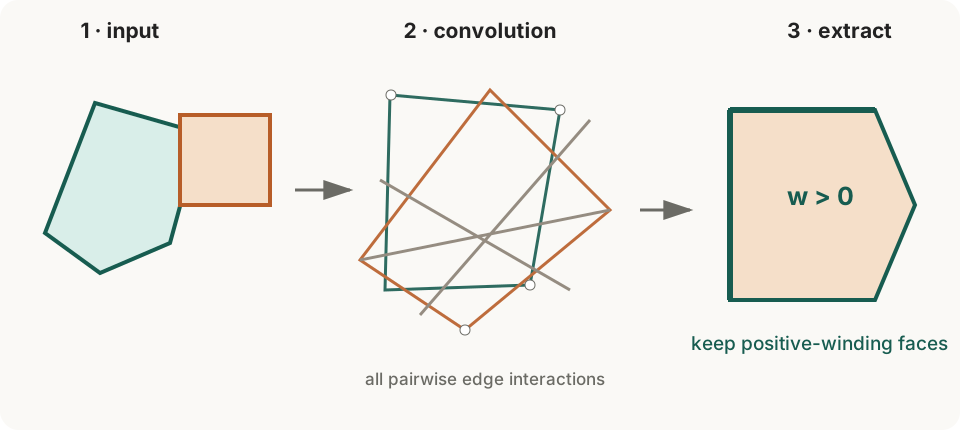
The main part of my thesis therefore uses the convolution method. Its essence is to construct a deliberately redundant arrangement first, and only then decide which parts belong to the Minkowski sum.

The algorithm in three ideas #

1. Combine boundary edges #

Take an oriented edge from polygon P and an oriented edge from polygon Q. Their vector sum describes a translated edge segment. By combining boundary edges according to their order, the algorithm builds a collection of segments called the convolution.

A useful way to picture this is to slide one edge along the other while preserving their directions. The resulting segments are not yet the answer. They are candidates for the answer’s boundary, and they may cross one another or enclose regions that should not be included.

For two simple polygons with n and m vertices, the convolution contains at most O(nm) segments before intersections are resolved.

2. Turn segments into a planar data structure #

The segments are split wherever they intersect and stored in a doubly connected edge list (DCEL). A DCEL records vertices, directed half-edges, their twins, the next edge around a face, and the face each edge bounds.

This data structure is the bridge between geometry and topology. Instead of asking complicated questions about every point, we can walk around each face of the arrangement and reason about its boundary. The implementation also has to handle coincident or overlapping segments—an unglamorous detail that becomes central when coordinates are represented by Java doubles.

3. Use winding numbers to select the result #

The convolution describes more than the Minkowski sum. The final step is a classification problem. For each face, the algorithm computes its winding number: informally, how many times the oriented convolution winds around a point in that face.

Faces with a positive winding number are the regions belonging to P ⊕ Q. Their boundaries are followed through the DCEL and assembled into the output polygon. In other words, the algorithm does not try to guess the final boundary while constructing it. It constructs all plausible boundaries, labels the regions, and filters the arrangement using a topological invariant.

That separation is the central idea of the thesis:

Geometry proposes the edges; topology decides which regions survive.

What made the implementation difficult #

The mathematical description is neat. The code is where the edge cases live.

I implemented and tested the algorithms in Java 8 using the ADSToolbox framework from the University of Bayreuth. Some practical lessons from that work have stayed with me:

• Normalize inputs early. Consistent orientation and removing redundant vertices simplify every later step.
• Avoid redundant objects. The convolution can grow quickly, so unnecessary allocations and repeated calculations become expensive.
• Choose data structures for the access pattern. In one part of the algorithm, random access to a sequence is important; a linked list would quietly turn a linear operation into a quadratic one.
• Treat floating-point equality as a design problem. Intersections that are theoretically identical may differ by a few bits. Comparisons, tolerances, and the order of operations all affect whether the DCEL is valid.
• Test topology, not only coordinates. A plausible-looking outline can still have the wrong orientation, a missing hole, or an incorrectly classified face.

The convolution method’s running time is bounded by O(n² · m²) for two simple polygons. That bound comes from the potentially quadratic number of intersections among the O(nm) candidate segments, plus the work needed to build and traverse the resulting arrangement. It is not the last word in Minkowski-sum algorithms, but it is a robust general method for the non-convex case considered in the thesis.

Looking back #

What I like about this project is that the final shape is the visible result of several layers of reasoning: vector addition, edge orientation, planar subdivisions, and winding numbers. None of those ideas is sufficient on its own. Together they turn a continuous geometric definition into a finite algorithm.

The obvious next step, which I identified in the thesis, is a reduced convolution. It uses topological properties to avoid constructing candidate segments that cannot contribute to the result. Fewer segments mean fewer intersections, less bookkeeping, and a better practical running time. Implementing and comparing that approach would be a natural follow-up project.

Writing this down years later also makes the broader lesson clearer: when a direct construction becomes messy, it can be more effective to build a rich intermediate representation and extract the answer from it with the right invariant.